Assignments & Grading

This course will make use of a variant of Specification Grading. This means that many assignments will be graded Complete/Incomplete or assigned a provisional grade, and in some cases will merely be returned with comments. Assignments marked Incomplete or not awarded full points may be revised and resubmitted. Quizzes can be retaken until passed, unless otherwise specified.

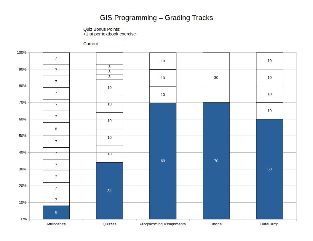
You will earn points along several tracks. Each track is worth up to 100 points. You must progress along ALL tracks to be successful in this course. Your final grade is based on the lowest score earned along any track.

Tracks proceed linearly and assignments usually need to be completed in the designated order. For example, for quizzes, the material is cumulative, and you can’t earn credit for Quiz 4 if you haven’t passed Quiz 3. Often, later assignments in a track presume knowledge you will have acquired by completing earlier assignments.

Some assignments proceed in milestones. In each case, you must proceed along the milestones in order. For example, for a term project, there will often be an initial topic statement, followed by an annotated bibliography (for a paper) or analysis plan (for an analytical project), a draft, and a final report. You cannot submit an annotated bibliography if your topic statement has not been approved, and you cannot submit a draft or final report if you haven’t submitted an annotated bibliography or analysis plan.

Grading will conform to the following scale:

A 93%+
A- 90 - <93%
B+ 87 - <90%
B 83 - <87%
B- 80 - <83%
C+ 77 - <80%
C 73 - <77%
C- 70 - <73%
D+ 67 - <70%
D 63 - <67%
D- 60 - <63%
F <60%

Attendance

0-100 points. Your attendance score is a straight percentage of class sessions you are present for.

This course meets once a week. Missing any class meetings will hamper your ability to complete the work in this course. High-performing students tend to be the ones who attend all class meetings. Struggling students may be struggling for a variety of reasons, but for many of them, lack of attendance is a contributing factor. Your attendance percentage will also indicate the maximum final grade you can earn in this course. If you miss 3 classes, you have attended 78.6% of class meetings. Accordingly, your final grade will not be higher than a C+, regardless of any other work completed.

An exception is that missing one class (attending 92.9% of class meetings) will still earn an A in the Attendance Track.

Quizzes

34 (base score) + 10 points for each of Quiz 1-5 + 3 points for each of Quiz 6-8 + bonus points.

Each topic will conclude with a short, graded programming quiz, beginning with the third week of class. The difficulty level should be comparable or easier than the weekly exercises, so if you complete the exercises, are present for in-class review, and review the exercises afterwards, you should be well-prepared for the quizzes.

The quizzes will be taken outside of class time. You may use the lecture slides, textbooks, and your own notes during the quiz. I strongly recommend using a printed “cheat sheet” of Python commands and functions. You may not use web searches, other people (including other students in the class), or other outside resources.

Your response to each quiz will usually be a single Python script which you upload to Canvas.

The quizzes are cumulative. Solving Quiz 5 will use knowledge demonstrated on Quizzes 1-4. Accordingly, you cannot earn points for later quizzes unless you complete all earlier quizzes.

Each week in the semester will be a quiz round. In a typical semester, quizzes will be due on a Thursday and graded on a Friday. If you do not pass a quiz, it will be unlocked for an additional attempt. You will keep taking the quiz until you complete it. When you complete it, you will earn full points for it. There is no penalty for requiring multiple attempts to pass a quiz.

In a week where you have to retake a quiz, you may also take the next quiz in sequence. That is, if you have to retake Quiz 2, you can also take your first attempt at Quiz 3. You may not take Quiz 4 or higher. If you fail Quiz 2 and Quiz 3, you will need to concentrate on completing Quiz 2. You will not get an additional attempt at Quiz 3 until Quiz 2 is completed successfully.

If you don’t take any quizzes one week, you have given up one opportunity to progress on the track. The final week of classes will be the last quiz round.

Quiz 1-5 (10 points x five)

Quiz 1: Python Basics, Strings
Quiz 2: Python Basics, Math
Quiz 3: Lists
Quiz 4: Conditional Evaluation
Quiz 5 Loops

Quiz 6-8 (3 points x three)

Quiz 6: Dictionaries
Quiz 7: Defining Functions
Quiz 8: Pandas Basics

Exercises (1/2 point x eight)

Each week during the first half of the course, exercises will be assigned from the textbook. The first handful are structured as practice quizzes (no points) in Canvas. Subsequent exercises involve modifying or creating short Python scripts. One question each week will be evaluated and bonus points awarded in the quizzes track for correct answers. The exercises must be submitted on time. Solutions will be posted to Canvas, so that you can check your work on questions that were not evaluated. We will review some of the exercises at the beginning of the class after the due date.

DataCamp

60 (base score) + 10 for each DataCamp course completed.

This course will make use of online exercises provided by DataCamp. You must use your Temple email address to register for a premium account (free using a link provided by the instructor). You will be required to complete three assigned DataCamp courses, and one additional one of your choosing.

The three required courses are broken up by chapter in Canvas, so that, for example, it is suggested that you complete “Ch 4 Loops” from the DataCamp Intermediate Python for Data Science course when we are reading “Ch 10 Repetition: Looping for Geoprocessing” and “Ch 11 Batch Geoprocessing” in the textbook. In some cases that means that I have assigned the DataCamp chapters out of order. Since the only thing you turn in is the course completion certificate, you may choose to progress through the course in the DataCamp order, as long as you complete all chapters on time.

You are required to complete the following courses:

Introduction to Python due during Module 3 – ArcPy Tools.
- Ch 1 – Python Basics should be completed during Module 1 – Python Basics
- Ch 2 – Python Lists should be completed during Module 2 – Lists and Tuples
- The remaining two chapters must be completed during Module 3 – ArcPy Tools
Intermediate Python due during Module 6 – Dictionaries
- Ch 3 – Logic, Control Flow and Filtering should be completed during Module 4 – Control Flow, Conditionals
- Ch 4 – Loops should be completed during Module 5 – Loops
- The remaining three chapters must be completed during Module 6 – Dictionaries
Python Data Science Toolbox (Part 1) due during Module 8 – Error Handling
- Ch 1 Writing your own functions and Ch 2 Default arguments, variable-length arguments and scope should be completed during Module 7 – User-Defined Functions
- The remaining one chapter must be completed during Module 8 – Error Handling

You will complete one additional DataCamp Python course of the your choosing. Suggested courses include:

You will have premium access to DataCamp courses for six months. You may choose to complete any additional courses you want to throughout the semester, and for a few weeks beyond the end of the semester.

Students who have previously used DataCamp and already completed the three required courses (the completion date on your DataCamp certificate is prior to this semester) should either retake the course if they feel they need a refresher or select another DataCamp Python course to do instead. Please ask me if you have any questions.

Programming Assignments

69 (base score) + 10 for each assignment.

These will be three short programming assignments that will build on material learned in the exercises and classroom demonstrations.

Programming Assignment 1 - Vector Analysis (10 points)

This assignment is based on Lab 6 - Vector Operations from GUS 5062 - Fundamentals of GIS. That lab exercises uses vector operations that you should be familiar with such as buffering, intersection, erasing, etc., to identify an area in Philadelphia suitable for a new store selling healthy foods. Many of you will have taken GUS 5062 and completed Lab 6 in ArcGIS. Now you will see how to automate it using ArcPy. For those of you unfamiliar with the exercise, reading the assignment at the end will give you a little more context.

The criteria for the target area, and the data sources necessary for the analysis, are:

In a Philadelphia Empowerment Zone. These are distressed urban areas targeted for reinvestment.
Within 2000 feet of a SEPTA High Speed Station or SEPTA Regional Rail Station.
NOT within 1200 feet of an establishment that already sells fresh produce, including Farmers Markets and stores participating in the Healthy Corner Stores Initiative.
A larger contiguous area is preferred to a smaller area.

Preliminaries

Begin by downloading all five shapefiles and unzipping them into a project folder. Unzip them so that all the shapefiles are at the same folder level. Do not have each shapefile in its own subfolder, as that will make referring to the file in code more verbose.

Your Python script should be saved and run in the same folder as the unzipped data files. When you run the script using Spyder, Spyder should set the working directory to the script directory. If it doesn’t, you can use the “Run configuration per file” dialog box (CTRL+F6) in Spyder to set the working directory to “The directory of the file being executed”. To make the ArcGIS workspace match your Python working directory, your script should being with:

arcpy.env.workspace = os.getcwd()

With your workspace set correctly, each shapefile can be referred to in code using a bare filename rather than a fully qualified path, e.g. “my_shapefile.shp”, not “C:/folder1/folder2/folder3/my_shapefile.shp”.

Analysis Plan

Begin by creating an inclusion layer. This should be the intersection of the areas that you want to include.
Then create an exclusion layer. This is the area that you do NOT want to include.
Use the exclusion layer to erase the non-desired areas from the inclusion layer.
In order to calculate the area of each candidate zone, first use the arcpy.MultipartToSinglepart_management tool to explode the resulting multipolygon; then use the arcpy.AddGeometryAttributes_management tool to calculate the area.
Find the area of the largest candidate zone. You can do this by opening the attribute table in ArcGIS. Put your answer in a comment at the end of your script. If you would like to do this step in code, you can try to do so by using a search cursor (PfA 17) or by using the arcpy.Statistics_analysis tool.

ArcPy Toolbox Functions That You Will Use

You will use the following ArcPy Toolbox functions in your analysis. Help for all these functions can be viewed within Spyder using CTRL+I, or by searching the documentation at ArcGIS.com. The names are specific enough that a Google search of, e.g., “ArcPy Buffer_analysis” will usually take you directly to the ArcGIS Pro or Desktop documentation for the tool. If the tool is discussed in the textbook, a page reference is given.

All of the following functions take as their first parameter a filename or list of filenames as inputs, and take as their second parameter an output filename that will get created on disk. They may have additional required or optional parameters.

arcpy.Project_management.
arcpy.Merge_management: PfA p. 101.
arcpy.Intersect_analysis: PfA p. 102.
arcpy.Buffer_analysis: First introduced in PfA on page 7 and used repeatedly for examples throughout the textbook.
arcpy.Dissolve_management.
arcpy.Erase_analysis.
arcpy.MultipartToSinglepart_management

Additionally you will need the arcpy.AddGeometryAttributes_managementtool. This function only takes an input file, which will be modified, as the first parameter (that is, no output file is specified). The required second parameter is the geometry attribute (or list of attributes) that you want to add. Use the following line of code to create a new field with the area of each feature. The new field will automatically be named POLY_AREA:

arcpy.AddGeometryAttributes_management("your_file.shp", "AREA")

Since the coordinate system units are feet, the area will be square feet unless you use specify a different unit.

Note that if you search the ArcPy documentation you will find that there are other ways of accomplishing the same thing, including CalculateGeometryAttributes_management and CalculateField_management. The tool I am suggesting is much easier to use, at the cost of being less flexible. For example, you have no control over the name of the created field, which is determined by the geometric measure that you calculate (area, length, centroid, point count, etc.)

Tips for Completing the Assignment

All of the data must be in the same projection. The downloaded shapefiles are all already in State Plane Pennsylvania South except the SEPTA Regional Rails Stations. You have to specify the output coordinate system when you call arcpy.Project_management, but keep in mind that you can pass the name of a .prj file to the out_coor_system parameter. All of the other shapefiles are in the desired coordinate system. Use the .prj from one of these files as input to this parameter. (Pay close attention to the filenames because the SEPTA High Speed Rail Stations are already in the correct coordinate system.)
In each case where you have to create a buffer, you need to buffer points from two different sources. It will be easiest if you merge the point layers first. Then you only have to run the buffer once. It will also be useful to use dissolve_option = "ALL" to dissolve the buffers.
Each toolbox function will create a new shapefile on disk. You can inspect these in ArcCatalog or add them to an ArcMap document to see your progress. If you add a layer to ArcMap, make sure to remove it before proceeding. ArcGIS file locking may prevent Python from being able to work with the file.

Deliverables

A script which completes all of these tasks.
The area of the largest contiguous zone that satisfies all criteria, either as a comment in the script, or printed to the console if you calculate it using ArcPy functions.
A map of the final layer of candidate zones (all candidate areas, not just the largest one). This map can be created in ArcGIS and exported to PDF. You do not have to make it pretty.

Grading

This assignment is worth 10 points, awarded 1 point for each of the following:

Create a script that runs to completion with no errors.
Set the ArcPy workspace correctly so that the script will execute successfully in a directory with the analysis data.
Use course coding conventions throughout.
Correctly reproject SEPTA Regional Rail Stations shapefile.
Correctly buffer Healthy Corner Stores and Farmers Markets shapefiles.
Correctly buffer SEPTA High Speed and Regional Rail Stations shapefiles.
Construct correct inclusion zone.
Correctly combine inclusion and exclusion zones.
Correctly add area field to singlepart result layer.
Provide adequate comments throughout your code.

Programming Assignment 2 - Spatial Data Catalog (10 points)

For this assignment, you will create a catalog of the spatial data available in the C:\gispy\data folder. This is the folder of data used for the textbook examples and exercises. You will construct a text file in Markdown, using Python’s file I/O functions, that stores the names of the workspaces, spatial layers, and some details of those layers.

In class we demonstrated the use of the os.walk method to recursively walk a folder tree, and the code we constructed is included below. ArcPy includes a similar iterator, arcpy.da.Walk. Whereas os.walk steps into each folder and lists each file, arcpy.da.Walk steps into each workspace and lists each spatial layer. A workspace could be a folder containing spatial data, but it could also be a geodatabase or other container. As you know, shapefiles are made up of multiple file system files. Whereas os.walk would list each shapefile part (DBF, SHX, PRJ, etc.), arcpy.da.Walk will list the complete shapefile once. DBF files will be listed if they are standalone tables, but will not be listed if they are part of a shapefile (that is, if the DBF has the same basename as an SHP file in the folder).

You will make liberal use of arcpy.Describe (see PfA 9.3) to extract information about each workspace and each spatial layer. Following the textbook, you can use the variable name desc when you instantiate the Describe object.

Markdown uses hashes (#) to indicate headings, with the number of hashes indicating the heading level. Use a first-level heading to print each workspace name and type, using the baseName and dataType method, respectively. Put the type in parentheses, and make sure to follow the heading with a blank line. Then print the path using the catalogPath method. The output Markdown should look like this:

# WorkspaceName (Folder, Workspace, etc.)

Path: C:\gispy\data\chxx\…

Use a second-level heading to print the name of each spatial layer (using the baseName method) in the workspace, followed by the data type in parentheses. Make sure to follow the heading with a blank line. Then print the path to the data using the catalogPath method. Your Markdown should look like this:

## LayerName (ShapeFile, TextFile, RasterDataset, etc.)

Path: C:\gispy\data\chxx\…

If the spatial layer is of type "RasterDataset", list the format on its own line:

Format: xxxxxx

If the spatial layer is a vector data type, list its geometry type (using the shapeType attribute:

Geometry Type: Point, Line, Polygon, etc.

If you attempt to read the shapeType attribute of a Describe object that is missing that attribute, Python will throw an error, so you only want to read this attribute for a vector layer. But there are several different vector data types. Rather than compare the value desc.dataType against a list of vector data types, it will be easiest to use the hasattr function to check whether the current Describe object has a shapeType attribute:

if hasattr(desc, "shapeType"):
    print(desc.shapeType)

If the layer has a fields attribute (again, use the hasattr function to check), output the name and data type of each field after a third-level heading “Fields”. (If the layer has no fields attribute, output “None” in bold.) The fields attribute returns a Python list of field objects. You will have to iterate this list and access the name and type attribute of each field object. Output the name of each field in bold, followed by a colon. Your Markdown should look like this:

### Fields

* **field1**: Integer
* **field2**: text
etc...

The spatial catalog should be created by a function that takes as parameters the path to top-level directory to walk and the name of the output file. The target directory should default to the current directory. The output file name should default to “catalog.md” in the same directory as the one being catalogued.

After defining the function, the function should be called with something like:

my_catalog_function("c:/gispy/data", "my_spatial_data_catalog.md")

If you find that you are having trouble completing the assignment using a function, start by creating it as a script. Define variables for the target directory to catalog and the output file name at the top of the script (after all of your imports).

The script should create a file using the file open function. This was demonstrated in class, and the script that was demoed is provided below. Make sure to use file.close() at the end, or make use of a with block as demonstrated in PfA 19.1.1.

Your script does not need any printed output, as the catalog itself is being written to a file. But if you have trouble with the file I/O, generate all Markdown in print functions so that you can earn points for those tasks (see Grading below). Other than that, if you want to, you could use print to output status messages like “Currently cataloguing ...".

Tips for Completing the Assignment

Start your assignment in a fresh script, which should be empty except for our usual imports.
Follow course coding conventions, including using snake_case for variable and function names, putting all imports at the top, etc.
Comment your code. Briefly describe what a variable or object is, what a for-loop is iterating or intended to do, what each output statement accomplishes.
Do not use command lines arguments (sys.argv) to control the script.
Assume the script will be run on a Windows computer with a correctly configured ArcPy environment, and with a data folder at c:\gispy\data.
Keep in mind that unlike the print function, the file.write method does not end with a newline! Thus, you have to add "\n" yourself for every write operation that you want to end with a newline. If you want a write operation to be followed by a blank line, you have to add two newlines ("\n\n") at the end.
There are many ways to build a text string in Python. I strongly recommend that you use f-strings. It has been demonstrated repeatedly in class, so you should have the most practice with it.
The Describe object has different attributes depending on the type of spatial data. Checking the dataType will give you a clue as to what attributes to expect, or use the hasattr function as described above.
Remember to use the from future imports. In particular, make sure to use Python 3 style printing if you have any print output in your script.
Remember to start small. Your first step should be a script that runs without errors even if it doesn’t do very much! Assigning variable names, or stubbing a function that doesn’t do anything is a good start. You can build up the script largely following the flow of the assignment. That is, first output names of workspaces. When that is working, then try to output spatial layer (file) names. When that is working, then try to output spatial layer characteristics. Make sure that each new addition generates working code before moving on to the next step.

Grading

This assignment is worth 10 points, awarded 1 point for each of the following:

Create a script that runs to completion with no errors.
Use course coding conventions throughout.
Call arcpy.da.Walk on the correct directory.
Generate correct Markdown for each workspace.
Generate correct Markdown for the name and type of each spatial layer.
Generate correct Markdown for additional attributes of each spatial layer.
Generate correct Markdown for all fields in each spatial layer that has fields.
Create a text file in the correct directory (root of the directory you are cataloguing).
Write correct Markdown to the text file created, with blocks in the correct order and blank lines separating each block.
Provide adequate comments throughout your code.

References

os.walk: PfA 12.4 and see below
arcpy.da.Walk: Ch 12 arcpyWalkBuffer.py sample script; PfA 15.3.2
The Describe object: PfA 9.3
Working with file objects: PfA 19.1 and see below
Markdown: https://guides.github.com/features/mastering-markdown/; you will only need the basic syntax for this assignment, not the Github Flavored Markdown extensions

Code Example

In class, we demoed using os.walk to recursively walk a folder tree, and using Python’s file input/output methods to write information about the folder contents to a file. A similar script is included here for your reference:

import os

folder_name = "c:/gispy/data/ch05"

fout = open("c:/gispy/scratch/list_files.txt", "w")

for current_folder, folders, files in os.walk(folder_name):
   
    fout.write(f"# {current_folder}\n\n")

    for i, filename in enumerate(files):
        print(os.path.join(current_folder, filename))
        fout.write(f"{i + 1}. {filename}\n")
   
    fout.write("\n")
   
fout.close()

In class, we used the triple current_folder, folders, files to store the items returned by the os.walk iterator. Keep in mind that the textbook and most examples you will find online and in the Python documentation will usually use root, dirs, files. As with any for-loop, these variable names are arbitrary. You could just as easily use peter, paul, mary, but it would make your code somewhat hard to understand. Using widely accepted conventions is usually a good idea.

Programming Assignment 3 - Analysis Automation (10 points)

For this assignment, you will create a script which, broadly, accomplishes the following steps using ArcPy.

Download and organize data locally - Fetching and unzipping data is covered in section 20.2 of the textbook.
Perform some kind of geospatial processing using ArcPy functions. Common geospatial operations such as buffering, nearest neighbor, zonal statistics, etc., can be considered.
Creates post-processing output: this could be a map, or a report with embedded map images - Map creation is covered in chapter 24 of the textbook.

The spatial operations should be motivated by a specific problem statement, and suitable data identified. As an example, consider the common geographic problem of areal allocation–the allocation of areal data to incommensurate geographies. You might want to determine demographics by Police District in Philadelphia, but Census tracts do not align with police districts. You have to determine the proportional area of each Census tract that falls in neighboring police districts, and allocate population to those districts. This would involve using arcpy.Intersect_analysis to construct the intersections and additional steps to calculate the areal proportions. A shapefile of Police Districts demographics would be created, and a choropleth map of the percent population with Bachelor’s degrees could be created.

The script should provide functions that do the following:

Download the necessary data. The script or scripts necessary to do this can be to a very large degree copied from Example 20.6 and 20.7 in the textbook.
Execute the spatial analysis. For the areal allocation example, a function could take the names of two data sources, the name of an output file, and a list of columns in data source 1 to allocate to the geographies of data source 2.
Generate the visualization of the output.

The script would then call these functions in order for a specific set of data.

Grading

The assignment is worth 10 points. Points will be awarded as follows:

(1 point) Create a script that runs to completion with no errors.
(1 point) Use course coding conventions throughout.
(2 points) Create a function that successfully downloads the data.
(2 points) Create a function that carries out the spatial analysis.
(2 points) Create a function that generates a map or report based on the output.
(1 point) Create a script which calls the functions in sequence for a specific implementation of the analysis.
(1 point) Provide adequate comments throughout your code.

Student-Led Python Package Tutorials

70 (base score) + up to 30 points as detailed below.

Students will work in teams of 3-4 to learn about a Python package and design a tutorial workshop to present to the class.

The tutorial should be structured as an approximately one hour workshop. The first few minutes can be devoted to an overview of the problem space. What business need are you trying to meet, or what analytical problem are you trying to solve? This may be accompanied by slides, but this is not a requirement, and definitely do not do several minutes of text-heavy slides. Following should be the workshop. This should be hands-on using Python scripts or Jupyter notebooks. The students should be given a workbook with clear instructions. You should live demo the code. Code should be clearly explained. And your team will circulate and help students with individual challenges.

The range of possible packages is quite wide. A list of packages of interest will be provided separately and discussed in class. Broadly, candidate packages are those used for spatial analysis, raster analysis, statistical visualization, geovisualization, and GIS-adjacent analyses such as machine learning and network analysis.

The team will need to read documentation, technical blogs, or other tutorials to learn about their topic, and then prepare their own tutorial workshop for the class. The workshop may be based on other tutorials that you find, but should be your own work. At the very least, you should make use of a different dataset than any tutorial that you consult when teaching yourself the topic. Try to use data of real-world interest to the class. Using data specific to Philadelphia or nearby regions is a good choice.

The workshop does not require Powerpoint. It can be entirely demo. If you do want to open up with an overview of the topic, keep it to five minutes max, and slides are still optional. Do not use slides for code.

Team members should rotate roles. Each person should have a chance doing teaching demo at the front of the room. Other team members should be circulating among the class, helping troubleshoot issues that the students are encountering.

Evaluation

(70 points) Base score.
(5 points) Team sends installation/data download instructions to the class at least 24 hours before their workshop.
(10 points) Tutorial workbook.
(10 points) Workshop is well-structured and leaves class with a useful first exposure to the topic.
(5 points) Team can knowledgeably respond to questions from the class.

Note that the workbook is the only part of the tutorial that can be revised. The rest of the requirements depend on preparing for and giving the workshop on the scheduled day. If the team is unprepared or outright misses the scheduled day, it cannot be made up.

Workbook

Your workshop should be accompanied by a workbook. The workbook should include things like package installation and data downloads. Packages should be installed using conda, not pip or other methods, unless you are demoing a package this is not available in a conda channel.

The workbook may include screenshots. Code should be included as text, not as a screenshot of a code editor! The workbook should also include links to documentation or learning resources related to your topic. These should be included in a reference section, but also consider including live links at appropriate points in the instructions.

I recommend that you construct your workbook in Markdown. You should export it to PDF and/or HTML. There are a number of converters that can do this, but a very easy one to use is RStudio, which you will also make use of in GUS 5162 and some of the PSM electives.

The workbook should have your names on it. This should be a document that you would feel comfortable posting publicly as a way to demonstrate your facility with these tools. It is also something that you would consider using to run a public workshop at a user conference or industry event.

Workshop

The workshop itself should be practical, and focused on accomplishing a particular outcome, which may be a data management outcome or an analytical outcome. Walk the students through steps to learn how to accomplish the goal. Examples should be clearly explained. Consider having a small number of additional exercises at the end, for which answers are not provided.

During the workshop itself, you should provide live demos or code walkthroughs. Then, as the students work through the workbook, you should circulate among the class, answering questions and helping troubleshoot. Bring the class back together at the end, perhaps showing the final intended result, or showing a further analysis or procedure that interested students could pursue on their own.

Deliverables

Slides (if any) or presentation outline. These should be provided to Prof. Hachadoorian approximately one week before the tutorial. Slides can be sent via email (PDF preferred) or shared as Google Slides.
Preparation Instructions. Send instructions to the class for anything that has to be downloaded or installed at least 48 hours prior to the workshop.
Workbook. This should probably be about 10 pages of text. With screenshots, code listings, and sources, it could easily be over 20. The exact length is a little difficult to predict ahead of time.

GIS Programming

Assignments & Grading

Attendance

Quizzes

Quiz 1-5 (10 points x five)

Quiz 6-8 (3 points x three)

Exercises (1/2 point x eight)

DataCamp

Programming Assignments

Programming Assignment 1 - Vector Analysis (10 points)

Preliminaries

Analysis Plan

ArcPy Toolbox Functions That You Will Use

Tips for Completing the Assignment

Deliverables

Grading

Programming Assignment 2 - Spatial Data Catalog (10 points)

Tips for Completing the Assignment

Grading

References

Code Example

Programming Assignment 3 - Analysis Automation (10 points)

Grading

Student-Led Python Package Tutorials

Workbook

Workshop

Deliverables